Playing with a Soccer Database from Kaggle.com
Recently I’ve downloaded as a zipfile (36 MB) from data science community Kaggle.com.
This zipfile contains a single file, a 313 MB sqlite Database. Let’s take a peek what’s inside:
Create connection to football DB
library(DBI)
con <- dbConnect(odbc::odbc(), "well-sqlite-footballdb")
Read in R packages necessary to load the data:
# tidyverse packages
library(dplyr, warn.conflicts = FALSE) #
library(purrr)   # functional programming
library(stringr)
library(lubridate) # strings to datetime
library(ggplot2)
library(NHANES)  # US health data
data(NHANES)
theme_set(theme_bw())
The database consists of 7 tables. We’ll read in all of them although we need only one, the Player table, which contains basic data of ~10000 soccer players from the top leagues of 14 European countries. They are not strictly “European soccer players”, but players from all over the globe, competing in the European Leagues.
table_names <- dbListTables(con)

good <- !  str_detect(table_names, "sqlite_sequence")
table_names <- table_names[good]

# Import all tables as data frames, 308MB
# feasible with lots of RAM
walk(table_names,function(x) assign(x,
                                    dbReadTable(x, conn=con),
                                    envir = globalenv()))
dbDisconnect(con)
Tables in the Sqlite database:
##                     Rows Columns
## Player_Attributes 183978      42
## Player             11060       7
## Match              25979     115
## League                11       3
## Country               11       2
## Team                 299       5
## Team_Attributes     1458      25
The Player table lists the soccer players’ weights in pounds, and their height in Centimeters. I don’t know how the people who compiled the database obtained the weight data, but I think FIFA requires it for their records. We’ll calculate Body Mass Index, (bmi) for each player which is defined as
\[\mbox{Body Mass Index }{bmi}=\frac{height}{weight^2}\] and has m/kg^2 as the unit of measure, but we’ll omit this from now on.
We’ll also create three size classes, large players who are taller than 1.90 m, ‘medium’ size players who are between 1.75 and 1.90 m tall, and ‘small’ players who are less than 1.75m.
pounds_per_kg <- 0.453592

sizes <- c("large" = 190, "small" = 175)
Player %<>%
  mutate(birthday = ymd(as_datetime(birthday))) %>% # was string
  mutate(weight = weight * pounds_per_kg) %>%
  mutate(bmi = weight /((height/100)^2)) %>%
  mutate(size = factor(
          if_else(height >= sizes["large"], "large",
          if_else(height >= sizes["small"], "medium", "small"))))
I’ll also focus on the “large” class of players mentioned below, because the players are more well-known, at least in Germany.
Calculate a few values to make plots below more informative:
range_bmi <- Player %>%  select(bmi) %>% range()
med_bmi <- median(Player$bmi)

diff_bmi  <- range_bmi %>% diff() %>% ceiling()
rng_seas  <- range(Match$season)
np        <- nrow(Player)
Display raw histogram with absolute counts:
# function common to most plots
# following convention in H.Wickham's ggplot2 Book, Ch 12
decorate <- function(x) {
  list(
    ggtitle(
      "Body Mass Index of Soccer Players",
      subtitle = sprintf("%s Players from Europe's Top Leagues, 2008-2016\n", x)
    ),
    xlab("Player Body Mass Index"),
    theme(legend.justification = c(1.25, 0.95), legend.position = c(1, 0.95)),
    scale_fill_discrete(
      name = "Player Height",
      labels = c(
        sprintf(
          "> %s cm)",
          sizes["large"]
        ),
        sprintf(">= %s cm)", sizes["small"]),
        sprintf("< %s cm)", sizes["small"])
      )
    )
  )
}
Code for the second plot in the panel below, right half of figure:
playerhist <- Player %>%
  ggplot(aes(bmi, fill=size)) +
#    geom_histogram(alpha=0.5, bins = diff_bmi*2) +
    geom_histogram(alpha=0.5, bins = diff_bmi*2, position="identity") +
    #xlim(c(0,70)) +

    decorate(np) +
    geom_vline(xintercept=med_bmi, size=0.3,
               color="darkgrey") +
    annotate(geom = "text", x = 20, y = 1690,
           label = sprintf("median BMI: %.1f ->", med_bmi),
           color="darkgrey") +
    geom_vline(xintercept=25.5, size=0.3, color="darkgrey") +
    annotate(geom = "text", x = 27.5, y = 750,
           label = sprintf("<- BMI %.1f:\n \"overweight\"", 25.5),
           color="darkgrey")

# add size classes to NHANES data set
NHANES <- NHANES %>%
        mutate(size = factor(
                if_else(Height >= sizes["large"], "large",
                        if_else(Height >= sizes["small"], "medium", "small"))))
us_males <- NHANES %>%
        filter(Age >= 19 , Age <= 35, Gender == "male")
nusm <- nrow(us_males)
usmalehist <- us_males %>%
        ggplot(aes(BMI, fill=size)) +
        #    geom_histogram(alpha=0.5, bins = diff_bmi*2) +
        geom_histogram(alpha=0.5, bins = diff_bmi*2, position="identity") +
        ggtitle("Body Mass Index of US Males",
                subtitle = str_c(
                        sprintf("%s Persons, Aged 19-35, in 2009-2912", nusm),
                         "from the US National Health and Nutrition Examination Study",
                        sep = "\n")) +
        xlab("Body Mass Index") +
        #ylim(c(0,1500)) +
        theme(legend.justification = c(1.25, 0.95),
              legend.position = c(1, 0.95)) +
        scale_fill_discrete(name = "Height",
                            labels = c(sprintf("> %s cm)", sizes["large"]),
                                        sprintf(">= %s cm)", sizes["small"]),
                                        sprintf("< %s cm)", sizes["small"])))

gridExtra::marrangeGrob(list(playerhist, usmalehist), nrow=1, ncol=2, top = "")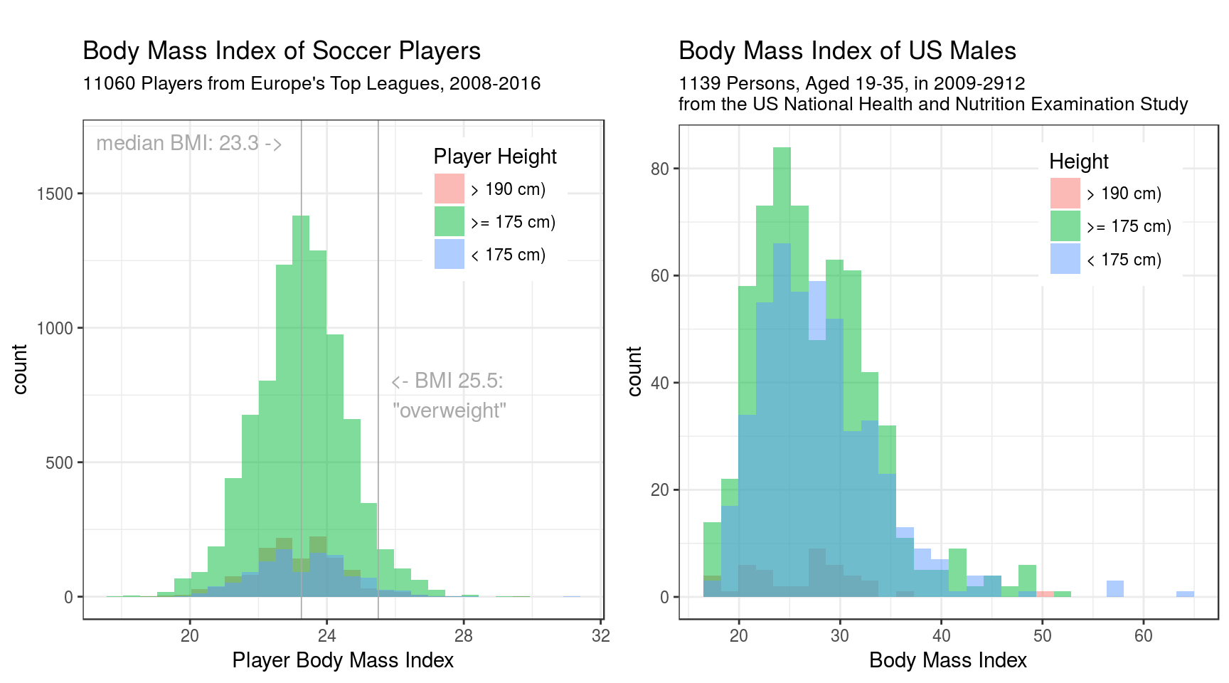
For comparison, I’ve added the BMI distribution of the general population, American males in this case. I’ve used the NHANES dataset, because it is available as a CRAN package, hence easily installed in R.
The axes in both plots are scaled differently, but I still prefer to have both plots side-by-side.
Of course the BMI range is much, much wider for the US men.
Who are the largest players with the highest BMI?
players_large <- Player %>%
  filter(size == "large") %>%
  arrange(desc(bmi))

# Top 6 PLayers
(players_large_top <- players_large %>%
                select(player_name, birthday, height, weight, bmi) %>%
                head())
## player_name birthday height weight bmi
## 1 Tim Wiese 1981-12-17 193 110.22 29.59
## 2 Marcus Hahnemann 1972-06-15 190 99.79 27.64
## 3 Ishmael Miller 1987-03-05 193 102.06 27.40
## 4 Hugo Almeida 1984-05-23 190 97.07 26.89
## 5 Christopher Samba 1984-03-28 193 99.79 26.79
## 6 Connor Ripley 1993-02-13 190 96.16 26.64Here I look up some more info about these high-BMI players. I’ll use my own (hidden) magic R function kgapi_lookup_kv() that looks up terms in the Google Knowledge Graph API which contains a large fraction of Wikipedia data, as a Linked-Data version.
players_large_top_kg <- map(players_large_top$player_name,
                            kgapi_lookup_kv)
Processing the column names is a bit messy, so this will not be shown here.
End result, see Table 1:
| Player Name | BMI | Short Desc | Long Description |
|---|---|---|---|
| Tim Wiese | 29.59 | Professional wrestler | Tim Wiese is a German professional wrestler and former football goalkeeper. |
| Marcus Hahnemann | 27.64 | Soccer player | Marcus Stephen Hahnemann is a retired American international soccer player of German descent. |
| Ishmael Miller | 27.40 | Soccer player | Ishmael Anthony Miller is an English professional footballer who is a free agent, having played most recently for Bury. |
| Hugo Almeida | 26.89 | Portuguese soccer player | Hugo Miguel Pereira de Almeida is a Portuguese professional footballer who plays as a centre forward for Croatian club HNK Hajduk Split. |
| Christopher Samba | 26.79 | Soccer player | Veijeany Christopher Samba, known as Christopher Samba, is a professional footballer who plays as a defender for Championship club Aston Villa. |
| Connor Ripley | 26.64 | English soccer player | Connor James Ripley is an English professional footballer who plays for Bury, on loan from Middlesbrough, as a goalkeeper. |
.jpg)
.jpg)
Surprisingly, German goalie Tim Wiese has the highest BMI. His career in the Bundesliga has ended, but he made some headlines in 2014-2016 because he did bodybuilding, and tried -temporarily- to pursue a career in Wrestling. See German Wikipedia.
His BMI is 29.6 m/kg². How large an outlier is this? Let’s plot some histograms:
vlines <- map(players_large_top_detail[, "BMI"], c) %>%  unlist()

Player %>%
  ggplot() +
  geom_vline(xintercept = vlines, linetype="dotted") +
  geom_histogram(aes(bmi, y = ..density.., fill=size), alpha=0.5, bins = diff_bmi *3) +
  decorate(np) +
geom_text(aes(x = BMI, y = -0.022, label = name), data = players_large_top_detail[1:4,], hjust = 1, vjust = 1, angle = 270) 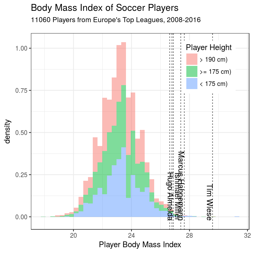
In the plot above, the BMIs of the players of table 1 are shown as dotted lines.
(Here the age classes have been stacked on top of each other, in contrast to the previous histogram with the US men)
dnorm_fit <- MASS::fitdistr(Player$bmi, densfun = "normal")

Player %>%
  ggplot(aes(bmi, fill = size)) +
  geom_density(alpha = 0.5) +
  stat_function(
    fun = function(x) dnorm(x,
                dnorm_fit$estimate["mean"],
                dnorm_fit$estimate["sd"]),
    color = "red",
    size = 0.5
  ) +
  ggtitle(
    "Body Mass Index of Soccer Players",
    subtitle = sprintf(
      "%s Players from Europe's Top Leagues,
      2008-2016. Mean BMI = %.1f m/kg², std.dev = %.1f",
      np, dnorm_fit$estimate["mean"], dnorm_fit$estimate["sd"]
    )
  ) +
  xlab("Player Body Mass Index") +
  # geom_vline(xintercept=dnorm_fit$estimate["mean"], color="red", size=0.2) +
  facet_wrap(~ size) +
  theme(legend.position = "none")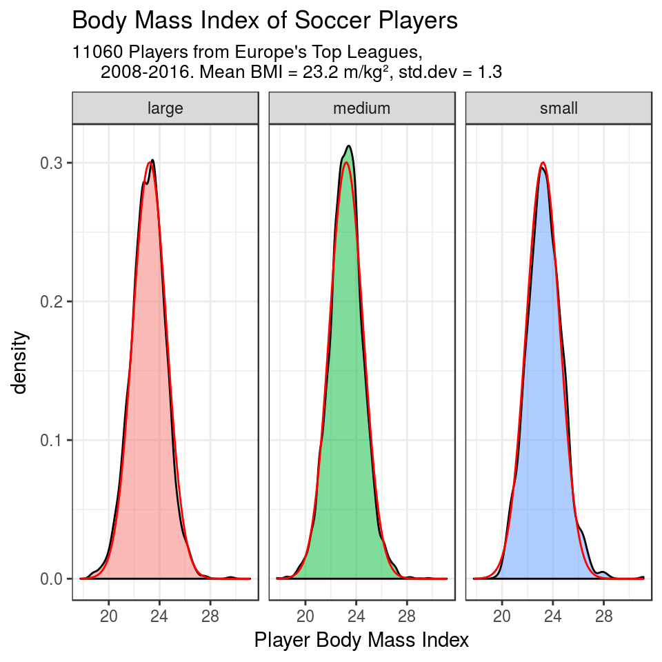
So we see that the BMI of soccer players in the top European Leagues fits pretty well a normal distribution with parameters mean = 23.2 and standard deviation = 1.3.
Appendix
This post is also available - maybe in a better, more readable version at my Github Repo for this site.
My blog: https://kbehrends.netlify.com.