Soccer-Database: Extracting goal data from XML fragments

Dataset

The dataset used here is the “European Soccer Database” - 25k+ matches, players & teams attributes for European Professional Football from Kaggle.com. This dataset is delivered as an Sqlite database. It contains 7 tables which have been populated by the original curator in 2014-2016. The data comes from many internet sources.

For the sake of brevity, I cannot repeat this information here. To see database internals, see the previous blogpost.

library(lubridate) # strings to datetime
library(tidyverse, warn.conflicts = FALSE)

theme_set(theme_bw())

The database consists of 7 tables. We’ll read in all of them. The Player table contains basic data of ~10000 soccer players from the top leagues of 14 European countries. They are not strictly “European soccer players”, but players from all over the globe, competing in the top leagues of certain Western European countries.

The problem

The problem I am solving here: Important information is stored inside the database, but the data is given in an unusable format. In this post I show how to transform the data content from these columns into a usable format.

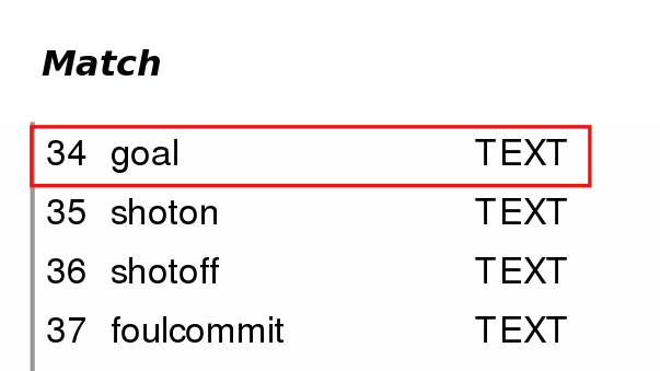
The “goal” column, which is column 34 in the “Match” table has a TEXT datatype:

This in itself is not a problem. However, an entry in this table typically looks like this:

library(xml2)
xmlparse <- function(s){
        read_xml(s) %>% 
                xml_find_all(".//player1")  %>% 
                xml_text()  %>% 
                str_c( collapse="\t")
}


# get 1 XML fragment for game 489042
xmlfrag <- Match %>% 
        select(match_api_id, goal)  %>% 
        filter(!is.na(goal)) %>% 
        filter(match_api_id == 489042) %>%
        select(goal) %>% 
        unique() %>% 
        rename("Goals for Game 489042:" = "goal") 

xmlout <- system(command = "tidy -q -i -xml ",
        input = as.character(xmlfrag), 
       intern = TRUE)

<goal>
  <value>
    <comment>n</comment>
    <stats>
      <goals>1</goals>
      <shoton>1</shoton>
    </stats>
    <event_incident_typefk>406</event_incident_typefk>
    <elapsed>22</elapsed>
    <player2>38807</player2>
    <subtype>header</subtype>
    <player1>37799</player1>
    <sortorder>5</sortorder>
    <team>10261</team>
    <id>378998</id>
    <n>295</n>
    <type>goal</type>
    <goal_type>n</goal_type>
  </value>
  <value>
    <comment>n</comment>
    <stats>
      <goals>1</goals>
      <shoton>1</shoton>
    </stats>
    <event_incident_typefk>393</event_incident_typefk>
    <elapsed>24</elapsed>
    <player2>24154</player2>
    <subtype>shot</subtype>
    <player1>24148</player1>
    <sortorder>4</sortorder>
    <team>10260</team>
    <id>379019</id>
    <n>298</n>
    <type>goal</type>
    <goal_type>n</goal_type>
  </value>
</goal>

This is XML text. The XML fragment was scraped from some website, and the curator of the database did not fully finish the job of parsing the information out of this. There is very detailed information (team ids; goaltype,…) inside, which is tedious to extract. And if the data was fully extracted, the new data would make the database design even more complicated, because more tables would be needed.

What does the XML text fragments contain?

With regard to the XML fragment, I think the <player1> element means this guy scored, <player2> made the assist.

These are the two <player1> we are interested in, with the following player_api_ids:

(scorer_api_ids <- xmlfrag  %>% 
        as.character() %>%
        xmlparse() %>%
        str_split(pattern =  "\t") %>% 
        unlist() %>% 
        as.numeric())

## [1] 37799 24148

I’ve looked it up for game 489042, Manchester United vs Newcastle, first PL game in Season 2008/2009, on August 17, 2008, the player IDs are correct.

Player %>% 
        filter(player_api_id %in% scorer_api_ids) %>% 
        select(player_api_id, player_name, birthday) %>% 
        mutate(birthday = format.Date(birthday, "%Y-%m-%d"))

##   player_api_id     player_name   birthday
## 1         24148 Darren Fletcher 1984-02-01
## 2         37799 Obafemi Martins 1984-10-28

These guys actually scored in that game.

Extracting goals from XML text

There are 25979 Matches in the database, and we have goal information for about 50% of them.

The goals can be extracted with this code:

xmlparse2 <- function(s){
                read_xml(s) %>%
                xml_find_all(".//player1") %>%
                xml_text(trim = TRUE) %>%
                str_c(collapse = "\t") %>% 
                str_c("")
}

# Parse xml and store result in tab-sep string
Match_Player_Goal <- Match %>%
        select(match_api_id, goal) %>%
        filter(!is.na(goal)) %>%
        filter(goal != "<goal />") %>%
        transmute(match_api_id = match_api_id,
                  goals_by = map_chr(goal, xmlparse2))

# assume there are no more than 20 goals per match
into <- map2_chr("Goal", 1:20, str_c)

# convert them into key-value table
Match_Player_Goal.2 <- Match_Player_Goal %>%
        separate(goals_by, into = into, "\t") %>%
        gather(k, player_api_id, -match_api_id) %>%
        filter(!is.na(player_api_id)) %>%
        mutate(player_api_id =  as.integer(player_api_id)) %>%
        arrange(match_api_id, k)

Add Player Names and Match names to this data frame:

Match_Player_Goal.3 <- Player %>% 
        select(player_api_id, player_name) %>% 
        right_join(Match_Player_Goal.2, by = "player_api_id") %>% 
        arrange(match_api_id, player_api_id) 

mplg_rds <- "data/Match_Player_Goal.3.RDS"
if(!file.exists(mplg_rds)){
 Match_Player_Goal.3 <- readRDS(mplg_rds)        
}

A few sample datasets from the new Match_Player_Goal.3 dataframe, which has 39872 rows:

head(Match_Player_Goal.3, 5)

##   player_api_id     player_name match_api_id     k
## 1         24148 Darren Fletcher       489042 Goal2
## 2         37799 Obafemi Martins       489042 Goal1
## 3         26181     Samir Nasri       489043 Goal1
## 4         30853 Fernando Torres       489044 Goal1
## 5         23139     Dean Ashton       489045 Goal1

Which player has scored the most goals?

#saveRDS(Match_Player_Goal.3, file="data_private/Match_Player_Goal.3.RDS")

Match_Season <- Match %>%
        select(match_api_id, season)

Player_most_goals <- Match_Player_Goal.3 %>%
        left_join(Match_Season) %>% 
        group_by(player_api_id, player_name, season) %>%
        summarise(goals = n()) %>%
        arrange(desc(goals)) %>% 
        ungroup()

Player_most_goals_season <- Player_most_goals %>% 
        inner_join(Player )

The following table is not particularly insightful; it just shows that I’ve more or less correctly parsed the XML-fragments in the datatable. We have 10629 players which shot 39665 goals in total, in 8 seasons.

Table 1: Goals per player and season

	season	player_name	goals	birthday	player_api_id
1	2011/2012	Lionel Messi	52	1987	30981
2	2014/2015	Cristiano Ronaldo	51	1985	30893
3	2011/2012	Cristiano Ronaldo	47	1985	30893
4	2012/2013	Lionel Messi	46	1987	30981
5	2014/2015	Lionel Messi	46	1987	30981
6	2015/2016	Luis Suarez	42	1987	40636
7	2015/2016	Zlatan Ibrahimovic	41	1981	35724
8	2010/2011	Cristiano Ronaldo	40	1985	30893
9	2015/2016	Cristiano Ronaldo	39	1985	30893
10	2015/2016	Gonzalo Higuain	36	1987	25759
11	2012/2013	Cristiano Ronaldo	35	1985	30893
12	2009/2010	Lionel Messi	35	1987	30981
13	2008/2009	Samuel Eto’o	33	1981	33639
14	2010/2011	Lionel Messi	32	1987	30981
15	2008/2009	Diego Forlan	32	1979	38460
16	2013/2014	Luis Suarez	32	1987	40636
17	2013/2014	Diego Costa	31	1988	19243
18	2011/2012	Robin van Persie	31	1983	30843
19	2013/2014	Cristiano Ronaldo	31	1985	30893
20	2012/2013	Edinson Cavani	31	1987	49677
21	2015/2016	Robert Lewandowski	31	1988	93447
22	2010/2011	Mario Gomez	30	1985	27326
23	2010/2011	Antonio Di Natale	30	1977	27734
24	2008/2009	David Villa	30	1981	30909
25	2015/2016	Lionel Messi	30	1987	30981
26	2012/2013	Zlatan Ibrahimovic	30	1981	35724
27	2011/2012	Klaas Jan Huntelaar	30	1983	36784
28	2009/2010	Antonio Di Natale	29	1977	27734
29	2009/2010	Didier Drogba	29	1978	30822
30	2011/2012	Wayne Rooney	29	1985	30829

Someone has counted Messi’s goals independently and found 52 goals, confirming the data listed in this table.

Goals per match

n_matches = n_distinct(Match_Player_Goal.3$match_api_id)
Match_Player_Goal.3 %>% 
        select(match_api_id, player_api_id) %>% 
        group_by(match_api_id) %>% 
        summarize(cnt_goals =n()) %>%
        ggplot(aes(cnt_goals) ) +
        geom_histogram(binwidth=0.5,  fill="navy") +
        ggtitle("Goals per Match", subtitle=sprintf("%s Matches with at least 1 goal", n_matches)) +
        xlab("Goals Count [per Match]") + ylab("Number of Matches")+
        theme(legend.position = "none") +
        scale_x_continuous(labels = 1:14, breaks=1:14)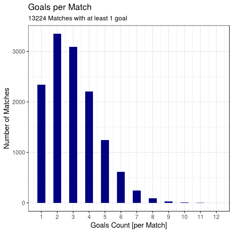

We can see that the curve peaks at 2 goals per match, but the curve is skewed to the right (fatter on the right half of the peak).

What is the average number of goals any player will score?

This is much more difficult to determine, because we don’t know how many times the player was in the squad but did not play, or when I was sick and could not play. Thus We only can calculate an average for players who have actually scored:

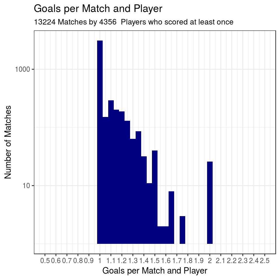
Note logarithmic scale on the y axis.

We see that even among those players who actually scored, the scoring average per match declines exponentially very quickly. Scoring 1.3 goals per match is very good, and 1.5 goals is extraordinary, very few players actually achieve this. (The peak at 2 goals per match and player is probably due to a few players who have played only in a single game but have shot two goals in that game.)

These numbers can be used as Priors for any subsequent Bayesian analysis. (TBC)