This is part 1 of a 3-part series of small blog posts about my first attempts at Bayesian Analysis of Soccer data. (Part 3 is not written yet).
In order to get started I had to invest much more effort than expected into cleaning the data and getting familiar with it.
Dataset
The dataset used here is the “European Soccer Database” - 25k+ matches, players & teams attributes for European Professional Football from Kaggle.com. This dataset is delivered as an Sqlite database. It contains 7 tables which have been filled by the original curator by scraping numerous websites many times in 2014-2016.
The SQLite database in question is a file on my local hard disk.
The database schema
The database schema can be viewed with the free schemacrawler tool.
Note: To get schemacrawler to work properly,
JavaandGraphvizneed to be installed on your computer. At this time, I do not know the minimum versions required for these tools. Just use the most recent relleases. Both are free.
A basic command to list the database contents is
# This is bash code for the unix command line
#
#  assign the absolute path to sqlite file to variable: db
db="/home/knut/code/git/football-data-collection/football-data.sqlite"
#
# the actual shell command
./schemacrawler.sh -server sqlite -database $db -password="" -c list
Output:
System Information
========================================================================

generated by                              SchemaCrawler 14.17.04
generated on                              2017-12-17 12:52:40


Tables
========================================================================

Country                                                          [table]
League                                                           [table]
"Match"                                                          [table]
Player                                                           [table]
Player_Attributes                                                [table]
Team                                                             [table]
Team_Attributes                                                  [table]
There are no views defined in the database.
List the table contents:
(This result is similar to the previous one, )
Row Count
========================================================================

Row Count
------------------------------------------------------------------------
Country                                                          11 rows
League                                                           11 rows
"Match"                                                      25,979 rows
Player                                                       11,060 rows
Player_Attributes                                           183,978 rows
Team                                                            299 rows
Team_Attributes                                               1,458 rows
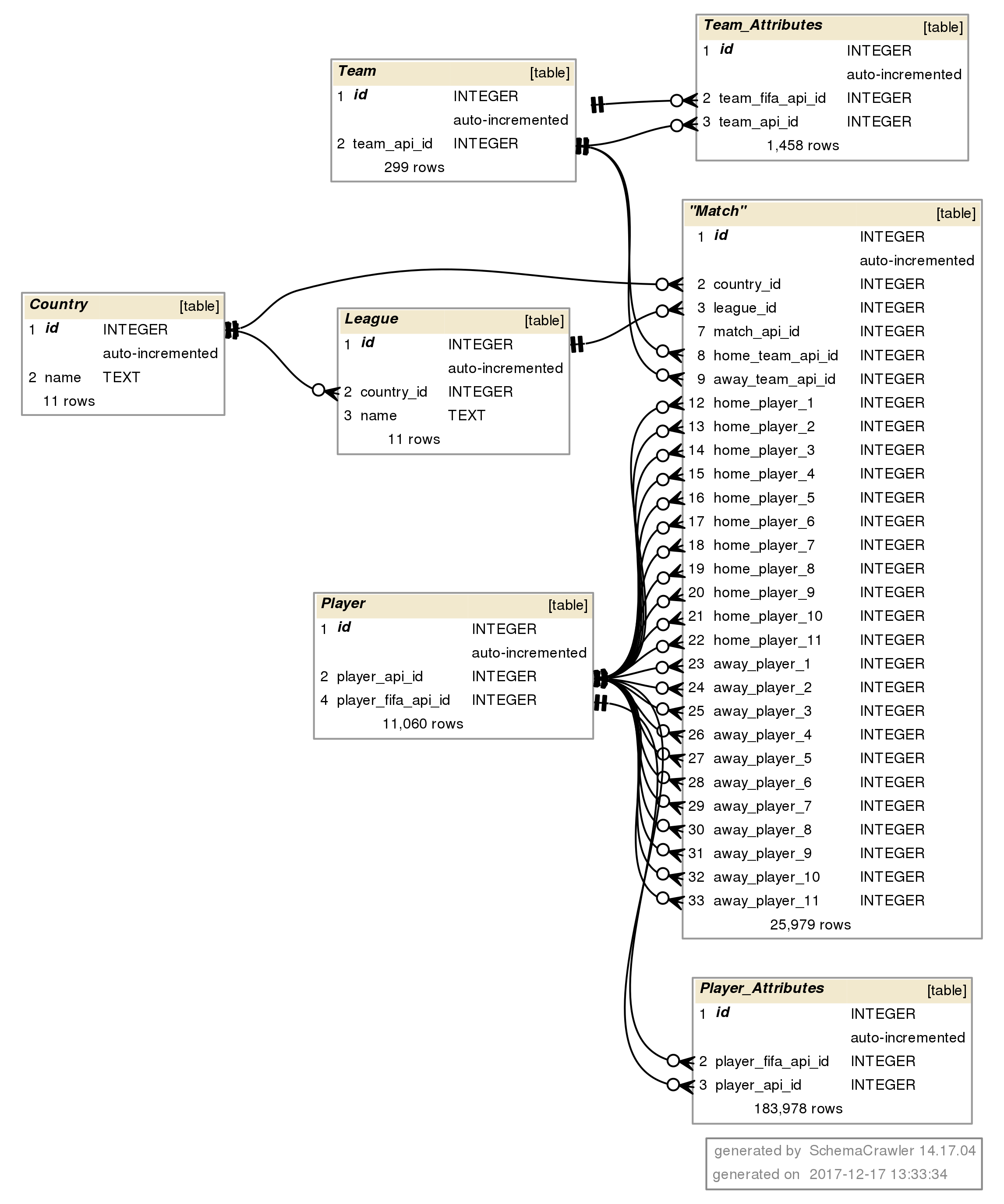
The “schema diagram”
Visualize these tables in a diagram, showing the tables, rowcounts, column names, columns datatypes, and their primarykey-foreignkey relationships between the tables.
As explained in the schemacrawler documentation, this can be done in many variants.
Command-line options used:
- To suppress schema names and foreign key names, use
-portablenames
- Show only significant columns, such as primary and foreign key columns, and columns that are part of unique indexes: use
-infolevel=standard -command=brief.
- optionally, to show column ordinals: set configuration option
schemacrawler.format.show_ordinal_numbers=truein the configuration fileconfig/schemacrawler.config.properties, as mentioned in the documentation
High-Level Diagram
This command can be used to create a PNG image file with a schema diagram.:
./schemacrawler.sh -server sqlite -database $db  -password="" \
   -infolevel=maximum -command=brief \
   -portablenames  -outputformat=png -outputfile=footballb--diagram--brief--no-constraintnames-colnum--rowcounts.png
This command yields this picture:
This diagram above is only high-level. A more accurate diagram would contain all nonempty columns in the tables and look like this:
“All relevant columns” diagram
The Match table contains a lot of columns from commercial betting companies. The 3-letter codes correspond to the odds and other bookie metadata.
“All columns” Diagram
The actual Match table contains many columns that serve no apparent purpose. There are dozens of columns that have names such as homePlayerX10, awayPlayPlayerY2…. The full diagram looks quite bizarre, and is shown here only for completeness:
./schemacrawler.sh -server sqlite -database $db  -password="" \
-infolevel=maximum -command=schema -portablenames  -outputformat=png \
-outputfile=footballb--diagram--with-playerXY-cols--no-constraintnames-colnum--rowcounts.png 

