Why this analysis?
There are two reasons:
- learn to process Twitter data at scale (~100MB-1GB/file - that’s large enough for me)
- get more info from/about the inspiring tweets from the CCC community
(This blogpost ist still a DRAFT - I want to publish quickly, even when an analysis is incomplete, or the text is a bit rough in places)
Background
Occasionally, over the last two years, I have gathered data from the Twitter Streaming API. However I have never really analysed these datasets.
Often my tweet-gathering happens during specific events, each with limited duration. When the period of data harvesting is limited to a few days or hours, data files do not get too big. For instance, I have collected tweets during the Euro 2016 Championship Final, during the US elections 2016, from the AGU/EGU geosciences conferences, and a few more. Until now these files just sat on my hard drive, untouched. They are typically less than 1 GB in size. For this study, I’ve used files 200 MB and 600 MB in size, containing tweets about the 33C3 and the 34C3 conferences, respectively.
I really like the Chaos Communication Congress), nicknamed XXC3. I remember well how I first happened to know about it, in 2003 or 2004. Waiting at a Berlin train station I saw that a high-rise building had become a giant light-installation (Projekt Blinkenlights). Baffled, I went to the conference center, purchased a ticket, and went inside. It was a great experience, so informative! (Back in those days, conference tickets were really easy to come by. Today ticket batches sell out within minutes, and are given preferably to CCC members and friends). Bitcoin, hardware hacking, security nightmares… I heard first about all these things, and many others, at the CCC congresses. During the last years, I didn’t attend any CCC conferences (maybe I’m too old for this…?)
Well, I never was a CCC member, and I’m not a really a hardware hacker or electronics guy. However, I think continued computer-education is important. Therefore I try to watch the live streams from the annual CCC conferences. Many of the streamed talks contain very high quality content, for free.
For a while now, I’ve also noticed that the tweets created during these conferences are highly inspiring. So let’s analyse the tweets a bit.
Preprocessing and simple timeseries plots
Load the necessary R packages, and the datafiles. (For details see github page).
Distribution of tweet lengths
Usually each tweet about any subject consists at least of 2000 characters. This might surprise you, because a tweet-text used to be 140 characters in length, until Twitter increased it to 280 characters in 2017. But a tweet contains a lot of metadata, and this makes a tweet exceed 2000 characters in length when serialized to a compact JSON string (not pretty-printed).
Line lengths of serialized tweet data-structures can be determined with:
awk '{print length}' stream_of_tweets.json > 34c3_strlength.txt .
The following histograms show that there were many more tweet data-structures for the 34C3 congress than for the 33C3 congress. There are also many junk tweet-fragments, from 0-2500 characters in length, that are not present in the 33C3 histogram (red rectangle).
I think the multi-modal peak structure of the histograms represents tweets that have been retweeted once or twice, or even more often. Actually I haven’t investigated that.
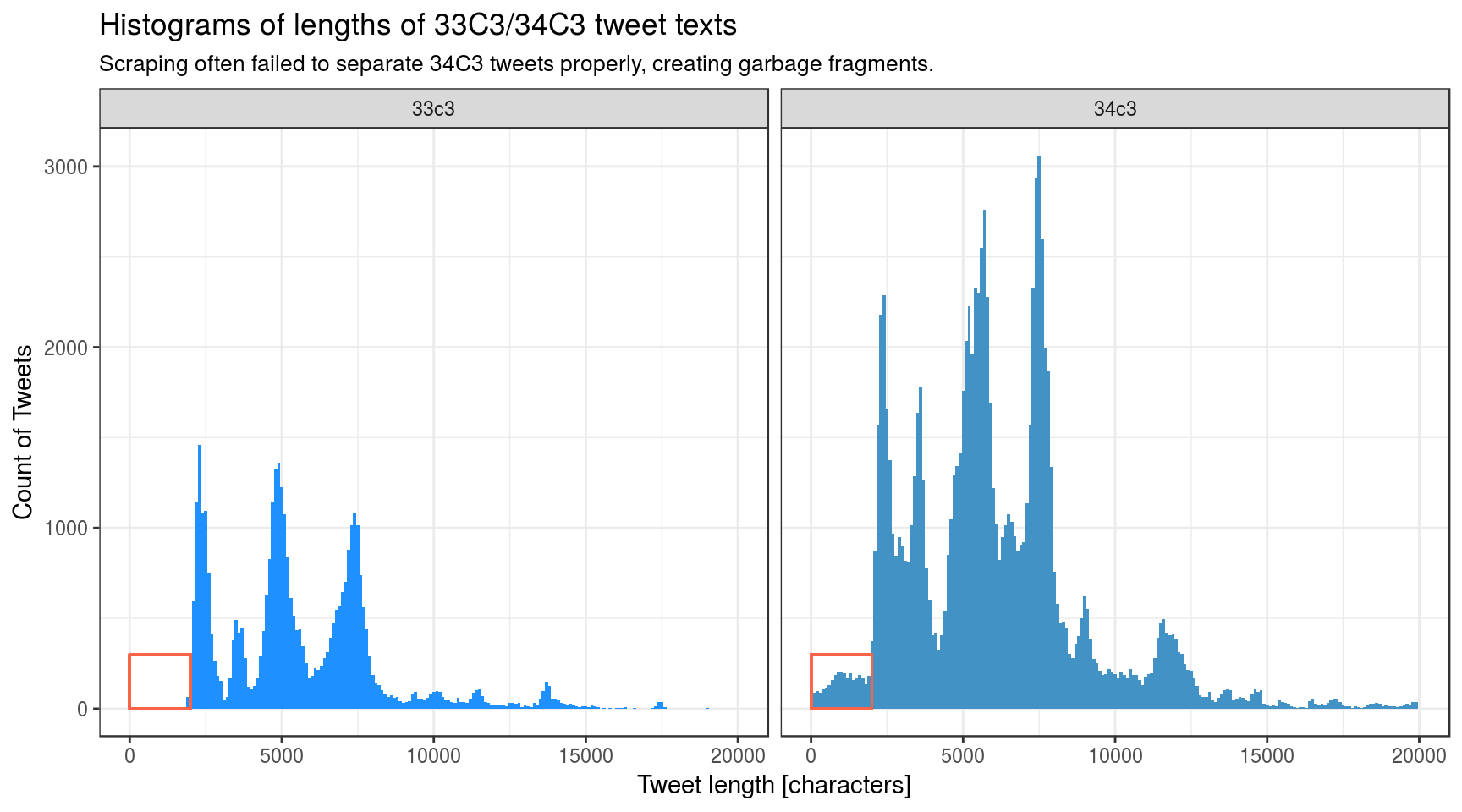
For 34C3, the harvesting script was not able to extract all tweets as syntactically valid JSON files. Visual inspection revealed that for some unknown reason they consist of many corrupted and duplicated tweets. I have not figured out exactly what was wrong. It seems that many tweets were nested inside each other randomly, but the nesting occured almost always on a single line. Still, some tweet fragments from the 34C3 scrape did span multiple lines; see the red rectangle in the figure above. However, there were so many garbage tweets in the 600MB .json-file that it was impossible to remove them all manually.
Bad JSON
So, what did the JSON look like? Not like this:
tweet1
tweet2
tweet3
tweet4
…but like this:
tweet1_tweet2fragment1
tweet2fragment2
tweet3
tweet4
Using a series of shell commands and pipelines, I tried my best to recover the first tweet from each line, discarding the fragmented JSON objects tweets misplaced and appended to each line. This recovery step might produce duplicated tweets for some reason.
Intermediate result:
tweet1
tweet1
fragment2
tweet3
tweet4
Valid tweets
Valid tweets always start with ‘“{created_at:”’, at the beginning of the line.
- keep these
- remove duplicated tweets
Thus I had to further preprocess the tweets with a command similar to this pipe:
grep  "^{\"created_at" stream__34c3.id_date_text.json |
   uniq > 34c3.created_at.json`
Convert dates to strings, group them into day-of-month, and hours-of-day.
Tweets gathered during the two events:
| Event | From | To | Num Tweets | Median Length of text |
|---|---|---|---|---|
| 33c3 | 2016-12-27 | 2017-01-01 | 37089 | 120 |
| 34c3 | 2017-12-21 | 2018-01-02 | 48709 | 127 |
There exist still more tweets about the 34C3 conference than about the 33C3, but the difference in tweet count is no longer as big as the first histogram above suggested.
Plot: User activity over time
This plot compares user activity on twitter during the 2 conferences, one year apart:
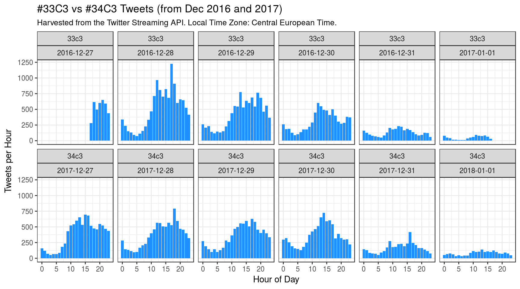
For the 33C3 I’ve started gathering tweets later (on Dec 27, 2016) and finished earlier, after 6 days. For the 34C3 I’ve let the script run unattended for 13 days (see also ‘Extra plots’, at end of post).
Observations (TBC)
The 34C3 congress had 15000 visitors, much more than 33C3 (12000), but absolute count of tweets per hour seems to be lower in 2017, during the first 2 days, whereas during the last 2 days users seem to have tweeted a bit more, though.
- Maybe Twitter has become less popular among the visitors?
- Maybe my preprocessing script was too aggressive in cleaning up things.
- Maybe the Twitter streaming API works differently?
(To be continued:)
- Wordcloud?
- Network Diagrams from mentions and retweets?
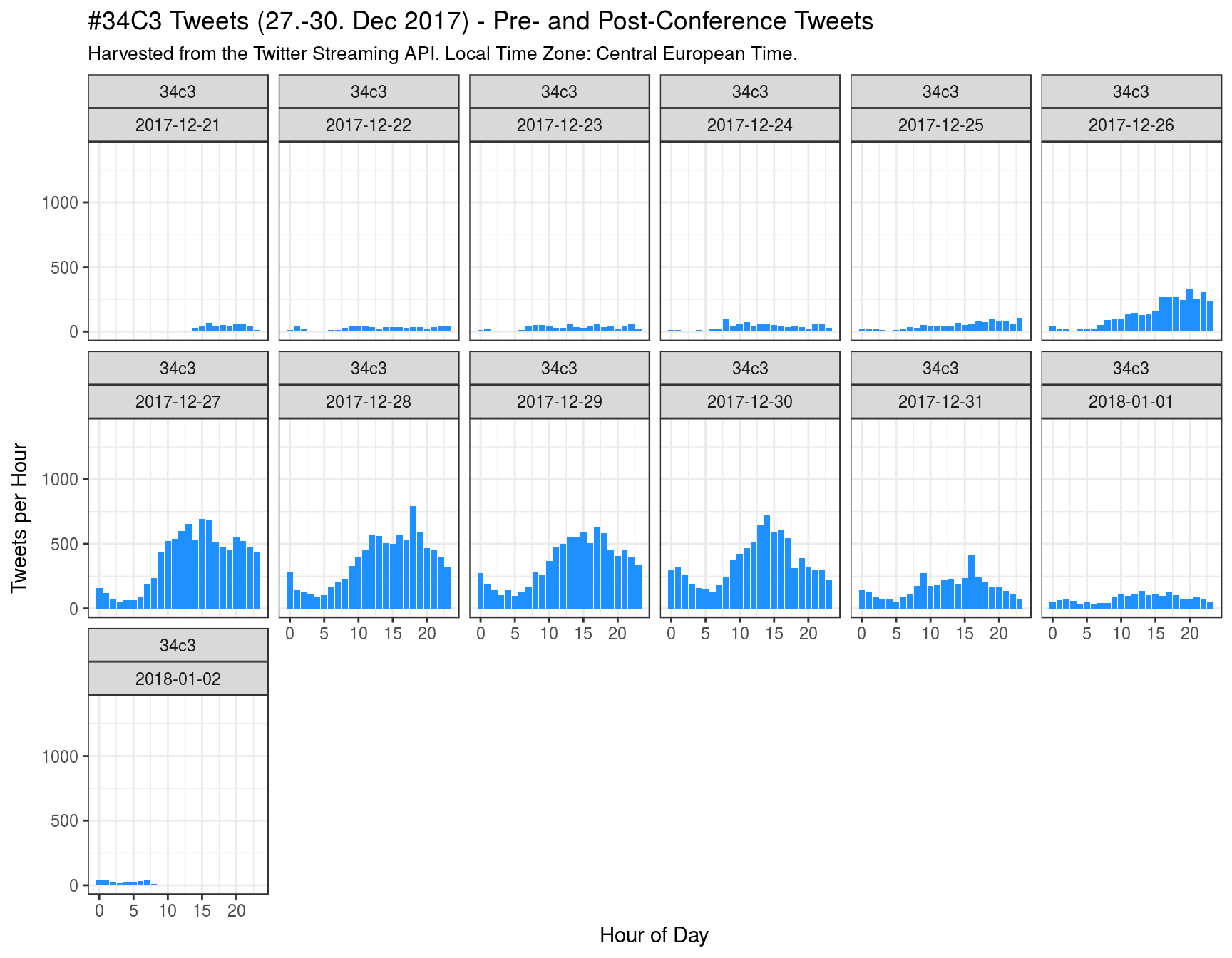
Extra plots
This plot shows that there was some user activity on Twitter even before the 34c3 started, and after it had ended.
(TBC)