Change of body parameters in soccer players
How did body mass index and body size of professional football players change over the years? Body size, not so much. It has stayed rather constant between 2008 and 2016. Average height might have even fallen a little bit. Body weight and, correspondingly, Body Mass Index on the other hand, have fallen even more. This means the top clubs want thinner players. It also means, in soccer, possibilities to increase the athleticism of players is limited.
As mentioned in previous blogposts, I’ve downloaded a zipfile (36 MB) with Football data from data science community Kaggle.com. The archive contained an SQLite Database.
library(DBI)
con <- dbConnect(odbc::odbc(), "well-sqlite-footballdb")
For the sake of brevity, to see the R packages I’ve included to process the data, see the previous blogpost. Only the tidyr package is new here.
library(tidyr) # gatherThe database consists of 7 tables. We’ll read in all of them. The Player table contains basic data of ~10000 soccer players from the top leagues of 14 European countries. They are not strictly “European soccer players”, but players from all over the globe, competing in the top leagues of certain Western European countries.
Tables in the Sqlite database:
##                     Rows Columns
## Player_Attributes 183978      42
## Player             11060       7
## Match              25979     115
## League                11       3
## Country               11       2
## Team                 299       5
## Team_Attributes     1458      25
The Player table lists the soccer players’ data.
Add some new attributes to the table.
pounds_per_kg <- 0.453592
sizes <- c("large" = 190, "small" = 175)

Player <- Player %>%
        mutate(birthday = ymd(as_datetime(birthday))) %>% # was string
        mutate(weight = weight * pounds_per_kg) %>%
        mutate(bmi = weight /((height/100)^2)) %>%
        mutate(size = factor(
                if_else(height >= sizes["large"], "large",
                        if_else(height >= sizes["small"], "medium", "small"))))

# from sqlite database foreign key constraints
#   FOREIGN KEY(`home_player_1`) REFERENCES `Player`(`player_api_id`),
The Match table contains data from 25979 matches, played between 2008-07-18 and 2016-05-25. The table contains 115 columns.
The names of the players comprising the teams are listed in 22 columns named home_player_1 to home_player_11, and away_player_1 to away_player_11. The substitute players nominated for the match are not known.
This database table has an untidy format. Let’s tidy it with the tidyr::gather() function:
Match_players  <- Match %>%
        select(match_api_id, season, league_id,
        home_player_1:away_player_11) %>%
        rename("match_id" = match_api_id)  %>%
        gather( k, player_api_id,  -match_id, -season, -league_id)
This table now looks like this:
head(Match_players %>% filter(!is.na(player_api_id)), 5)## match_id season league_id k player_api_id
## 1 493016 2008/2009 1 home_player_1 39890
## 2 493017 2008/2009 1 home_player_1 38327
## 3 493018 2008/2009 1 home_player_1 95597
## 4 493020 2008/2009 1 home_player_1 30934
## 5 493021 2008/2009 1 home_player_1 37990I’ve only shown 5 rows of this 571538 x 5 table. This table can now be joined with the Player table:
Player_in_match <- Player %>%
        inner_join(Match_players, by = c("player_api_id" = "player_api_id")) %>%
        mutate(year_of_birth = year(birthday)) %>%
        rename("player_id" = id)
We’ll start with body size, because it is an easier quantity to understand.
## there are too few players in the dataset
# born earlier than 1975, and after 1998
yob_thresh_max <- 1975
yob_thresh_min <- 1997


Player_height_by_year <- Player_in_match %>%
        select(year_of_birth, size, height ) %>%
        filter(year_of_birth >= yob_thresh_max) %>%
        filter(year_of_birth <= yob_thresh_min) %>%
        group_by(year_of_birth) %>%
        summarize( avg_height = mean(height))

# average body height seems to go down a little bit
Player_height_by_year %>%
        ggplot(aes(year_of_birth, avg_height)) +
        geom_point() +
        geom_smooth(method="loess", span=1, se=TRUE) +
        ylab("Average Player Height [cm]") +
        xlab("Player's Year of Birth") +
        ylim(c(175, 190))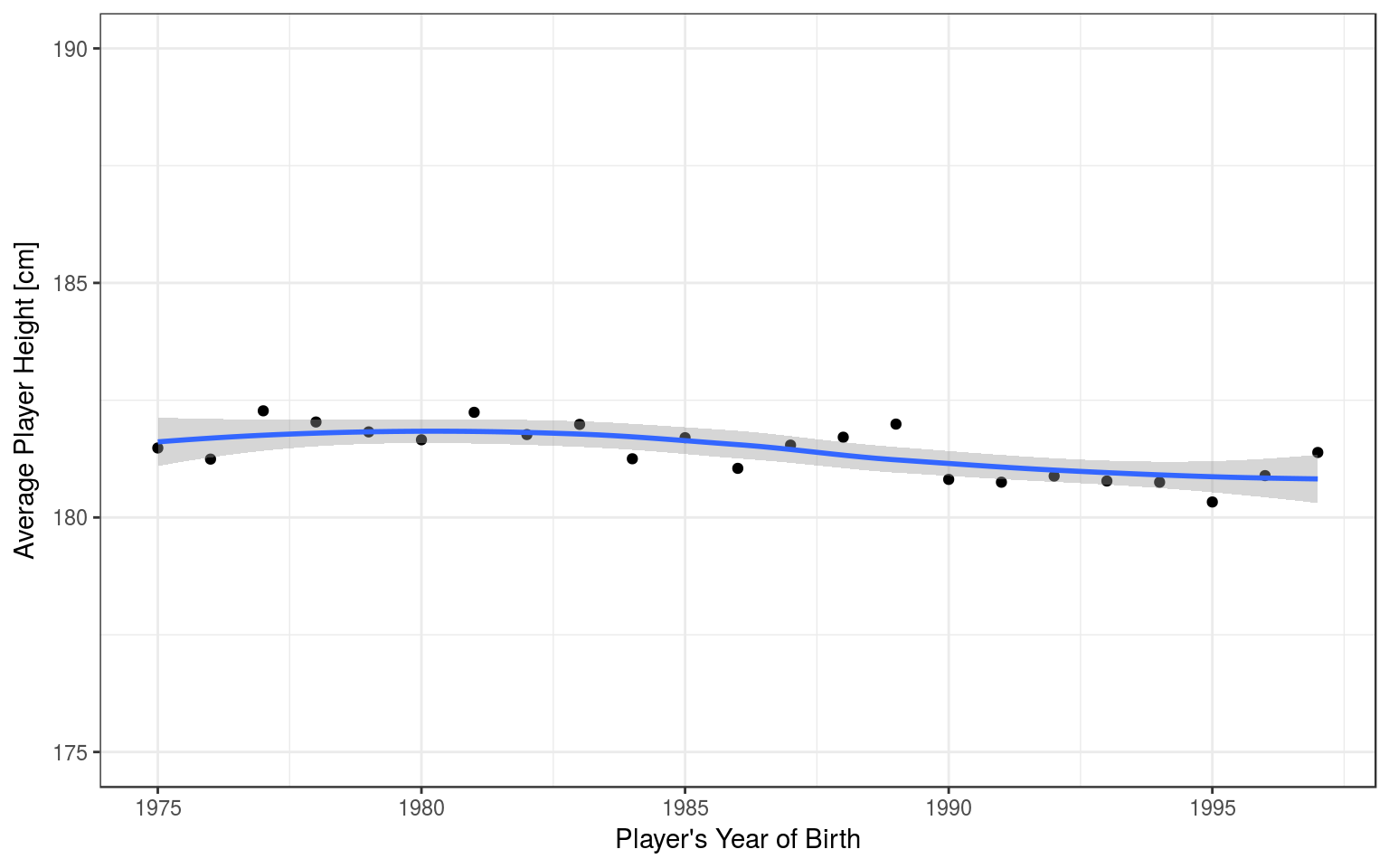
Average body size might have even fallen a bit in professional soccer. This trend is unlike Icehockey, where another data scientist has collected evidence in a blogpost that professional players have an average body size 183 cm in 2010, and this increases about 0.1 cm per year.
BMI per year
How did Body Mass Index change over the years?
The following plots show that BMI seems to fall. Maybe this is an artifact, because for the years 2016 the database contains much more younger players who are not fully grown up biologically and have less massive bodies.
Player_bmi_by_year <- Player_in_match %>%
        select(year_of_birth, season, player_api_id, bmi) %>%
        group_by(year_of_birth, season) %>%
        #        summarize(distinct_players = n())
        summarize(distinct_players =n_distinct(player_api_id)) %>%
        ungroup()


Player_bmi_by_year %>%
        group_by(year_of_birth) %>%
        summarize(distinct_players = sum(distinct_players)) %>%
        ggplot(aes(year_of_birth, distinct_players)) +
        geom_point() +
        geom_smooth(method="loess", se=FALSE) +
        ylab("Number of BMI by  Players in Database") +
        xlab("Players' Year of Birth") +
        geom_vline(xintercept = c(yob_thresh_max, yob_thresh_min),
                   color="maroon") +
        ggtitle("European Soccer Database: Players' Appearances in Matches",
                subtitle = "By year of birth. Double counted for each season. Seasons 2008-2016.")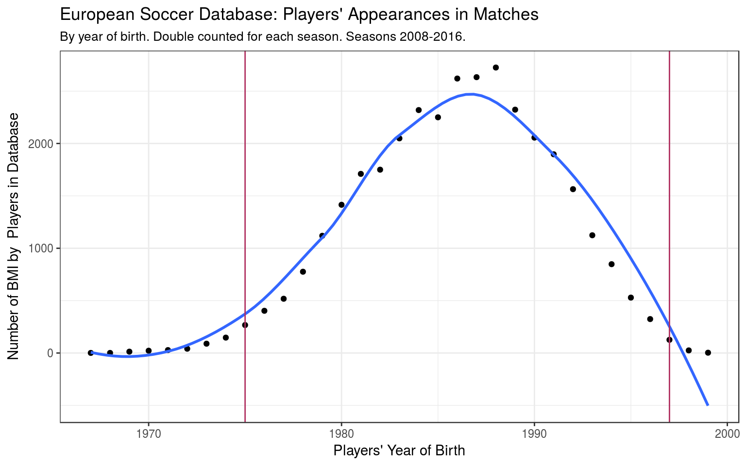
# remove players where we have too few counts
Player_bmi_by_year <- Player_in_match %>%
        select(year_of_birth, bmi ) %>%
        filter(year_of_birth >= yob_thresh_max) %>%
        filter(year_of_birth <= yob_thresh_min)

Player_bmi_by_season <- Player_in_match %>%
        select(season, bmi )

Player_bmi_by_year.2 <- Player_bmi_by_year %>%
        group_by(year_of_birth) %>%
        summarize( avg_bmi = mean(bmi))

# average BMI over the years
Player_bmi_by_year.2 %>%
        ggplot(aes(year_of_birth, avg_bmi)) +
        geom_point() +
        geom_smooth(method="loess", span=1, se=FALSE) +
        ylab("Average Player BMI") +
        xlab("Players' Year of Birth")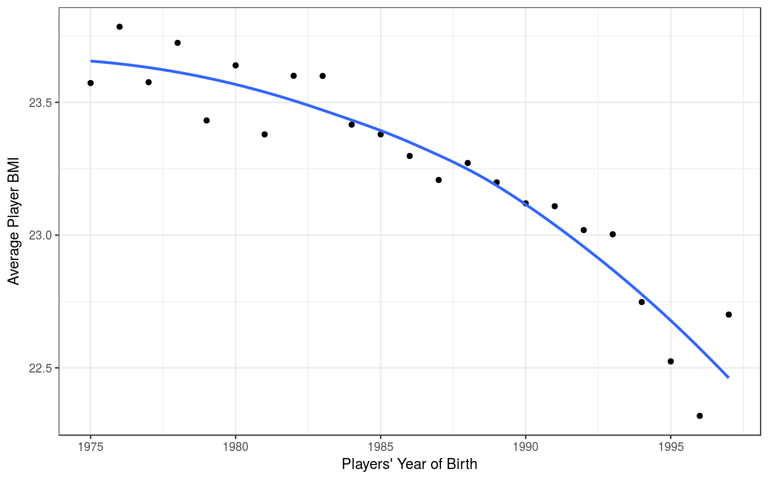
# 1 boxplot per year - trend is less obvious
Player_bmi_by_year %>%
        mutate(year_of_birth = factor(year_of_birth)) %>%
        ggplot(aes(year_of_birth, bmi)) +
        geom_boxplot() +
        ylab("BMI") +
        ggtitle("Body Mass Index of Soccer Players over years")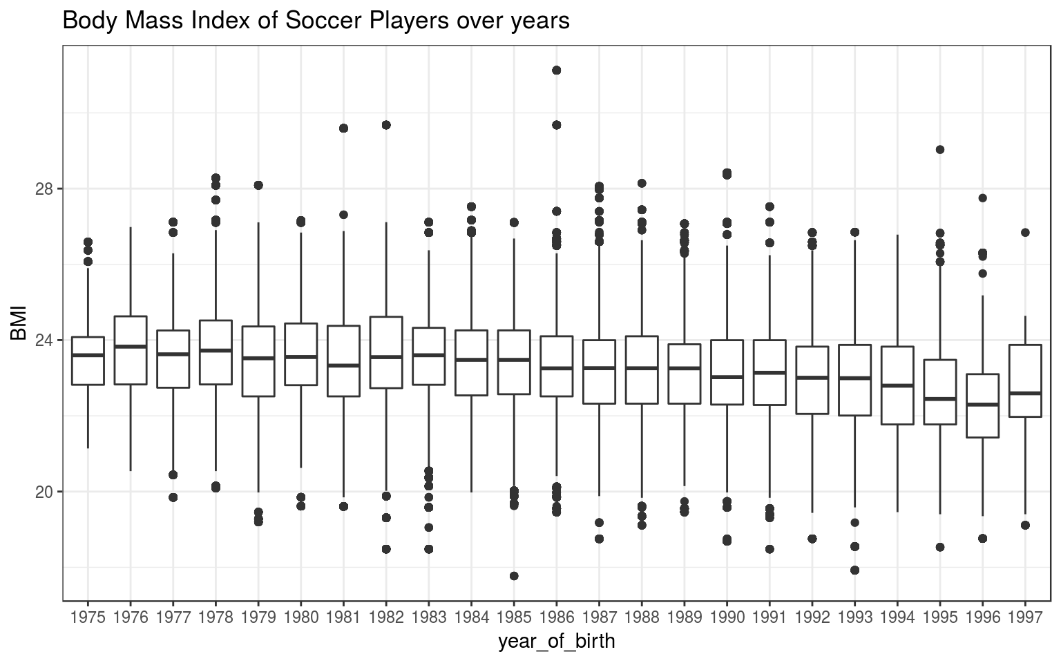
# BMI per season
Player_bmi_by_season %>%
        ggplot(aes(season, bmi)) +
        geom_violin() +
        ylab("BMI") +
        theme(axis.text.x=element_text(angle=60,hjust=1)) +
        ggtitle("Body Mass Index of Soccer Players over years")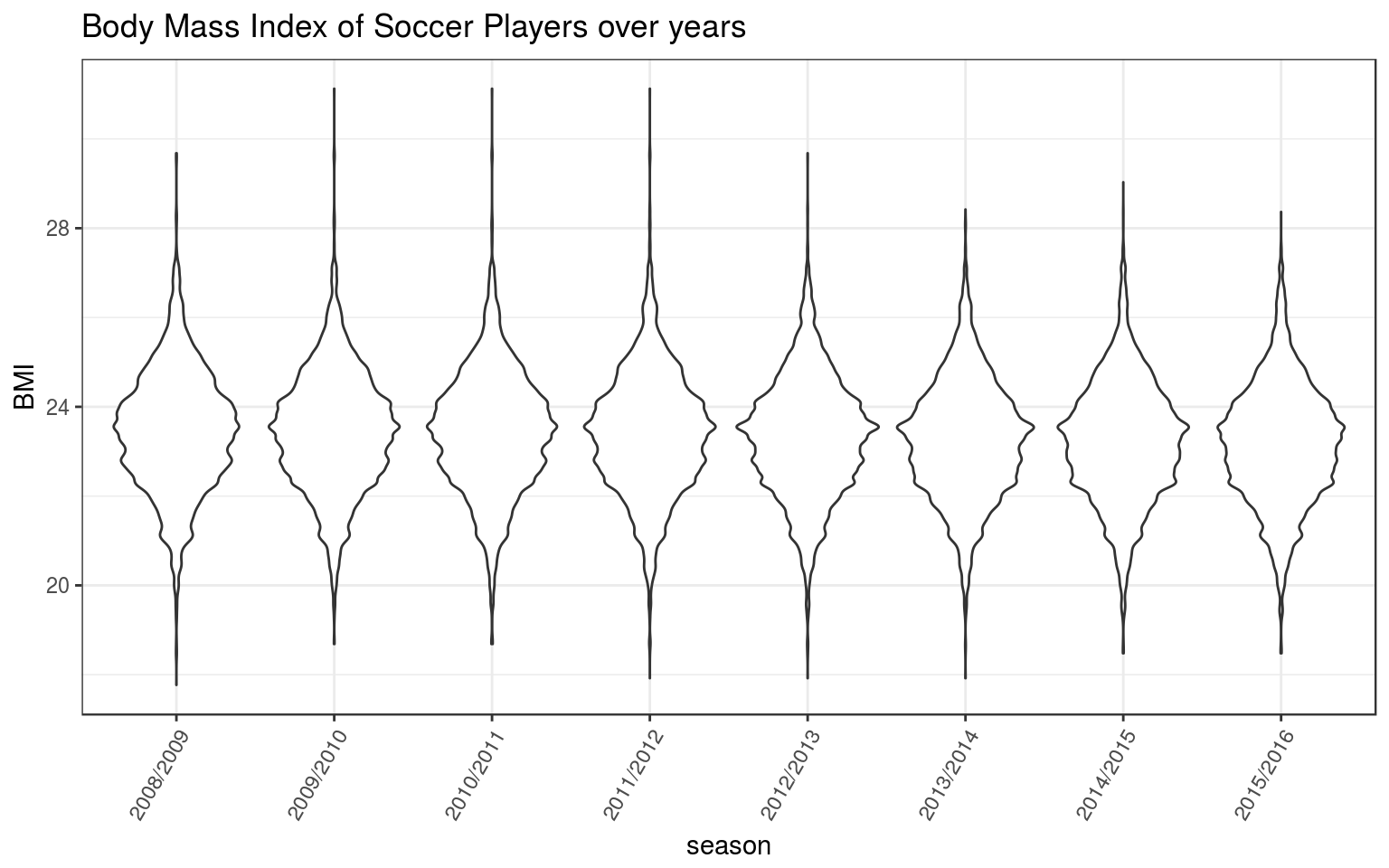
These violin plots show the distributions of players’ BMIs per season. They appear to be very much alike. You might think that the range of values goes down - indicating that players get more uniform with respect to BMI. I also think clubs prefer thinner, younger, more agile players. Or the residence time of players in clubs has gone down, or younger players get into top clubs at an earlier age.